After three years, this is my final day on the Talisman project as I start on the Future Cities Catapult project on October 1st. If you go back through the blog posts, all the project highlights are there, including all the builds, conferences, workshops, exhibitions and the hackathon.
Following on from my last post on running agent based models in MapTube using AgentScript, I’ve now got my “live” tube animation working:
I’ve speeded up the trains by a factor of 10 so you can see them move, but otherwise, it’s just a modification of the coffeescript code I was using before on a standalone web page. This isn’t on the production MapTube website yet, only the development tree as there are still a few problems to iron out. Also, it’s not really live as the data is loaded from an archive file stored on the same site. This highlights one of the problems with loading data dynamically. I could pull a live file straight off of the ANTS server which we use for all our live visualisations. The problem with this is that it’s a cross site request, so I’m going to need to put a JSONP endpoint into the server in addition to regular JSON and XML. The alternative would be to create a proxy on MapTube, but I’m trying to keep the code as generic as possible.
What’s happening at the moment is that the coffeescript model of the tube system is created just as though it were a normal standalone AgentScript model with no map behind it. The initialisation creates an “AgentOverlay” class which encapsulates the model and handles all the necessary interaction with the Google Map:
The “AgentOverlay” communicates with the MapTube code on the page to register the overlay which allows interaction with it. As you can see from the YouTube clip, the layers icons on the right hand side are still missing and I need to include some additional code so the model can pop up its own colour scale and other widget windows. At the moment it’s looking like it’s possible to give the code almost complete control over the information it shows, which will give me the ability to create custom maps very easily. The only issue that looks impossible to fix, though, is the separation of code between layers. There are always going to be code clashes between layers, so it’s just going to have to rely on programmers using unique namespaces for their code.
ModelTube is the name of the project to integrate agent based modelling into MapTube. Back at the end of last year I did a blog post on how to integrate AgentScript with Google Maps: http://www.geotalisman.org/2013/12/18/bugs-on-a-map/. Following on from this, I used the AgentScript agent based modelling framework, which is based on NetLogo, to visualise the tube network in real time: http://www.geotalisman.org/2014/04/29/another-day-another-tube-strike/. Visualisation of real-time data using agent based modelling techniques makes a lot of sense, especially when the geospatial data is already available on MapTube anyway.
The following image shows a variation of the “AgentOverlay” class added as a new map type in MapTube:
This is the same simple example of agents moving randomly around a map as in the “Bugs on a Map” example, except that this time it’s integrated into MapTube as a “code” layer. The idea of a “programmable map” layer that you can experiment with is an interesting idea. By allowing programmable map layers, users can upload all kinds of interesting geospatial visualisations and are not just limited to choropleths.
It’s going to be a while before this new map type goes live though, as there are still a number of problems to be overcome. The datadrop needs to be modified to handle the code upload, but the biggest problem is with the scripts themselves. The “bugs” example above is written in coffeescript, so I’m having to compile the coffeescript into javascript at the point where it’s being included into the page. I liked the idea of something simpler than Javascript, so I could give the user a command line interface which he could use to create a map with. Sort of like a JSFiddle for maps (MapFiddle?).
MapTube is actually quite clever in how it handles map layers. What it does behind the scenes is to take an XML description of the map layers and transform this into the html page that you see in the browser. This makes it very easy to implement a lot of complex functionality as it’s all just transformational XML to XHTML plus a big chunk of library code. At the moment, though, I’m stuck with how to separate code in different map layers, while still being able to call the layer’s initialisation and get the overlay back. Then there are the cross site scripting problems which are making it difficult to load the tube network and real-time positions. Hopefully, a real-time tube demonstration on the live server isn’t far away.
I’ve been experimenting with 3D buildings in my virtual globe project and it’s now progressed to the point where I can demonstrate it working with dynamically loaded content. The following YouTube clip shows the buildings for London, along with the Thames. I didn’t have the real heights, so buildings are extruded up by a random amount and, unfortunately, so is the river, which is why it looks a bit strange. The jumps as it zooms in and out is me flicking the mouse wheel button, but the YouTube upload seems to make this and the picture quality a lot worse than the original:
Performance is an interesting thing as these movies were all made on my home computer rather than my iMac in the office. The green numbers show the frame rate. My machine is a lot faster as it’s using a Crucial SSD disk, so the dynamic loading of the GeoJSON files containing the buildings is fast enough to run in real time. The threading and asynchronous loading of tiles hasn’t been completed yet, so, when new tiles are loaded, the rendering stalls briefly.
On demand loading of building tiles is a big step up from using a static scene graph. The way this works is to calculate the ground point that the current view is over and render a square of nine tiles centred on the viewer’s ground location. Calculation of latitude, longitude and height from 3D Cartesian coordinates is an interesting problem that ends up having to use the Newton-Raphson approach. This still needs some work as it’s obvious from the movies that not enough content ahead of the viewer is being drawn. As the view moves around, the 3×3 grid of ground tiles is shuffled around and any new tiles that are required are loaded into the cache.
Working on the principle that tiles are going to be loaded from a server, I’ve had to implement a data cache based on the file URI (just like MapTubeD does). When tiles are requested, the GeoJSON files are moved into the local cache, loaded into memory, parsed, triangulated using Poly2Tri, extruded and converted into a 3D mesh. Based on how long the GeoJSON loading is taking on my iMac, a better solution is to pre-compute the 3D geometry to take the load off of the display software. At the moment I’m using a Java program I created to make vector tiles (GeoJSON) out of a shapefile for the southeast of England. I’ve assumed the world to be square (-180,-180 to 180,180 degrees) then cut the tiles using a quadtree system so that they’re square in WGS84. Although this gives me a resolution problem and non-square 3D tiles, it works well for testing. The next step is to pre-compute the 3D content and thread the data loading so it works at full speed.
Finally, this was just something fun I did as another test. Earth isn’t the only planet, other planets are available (and you can download the terrain maps)…
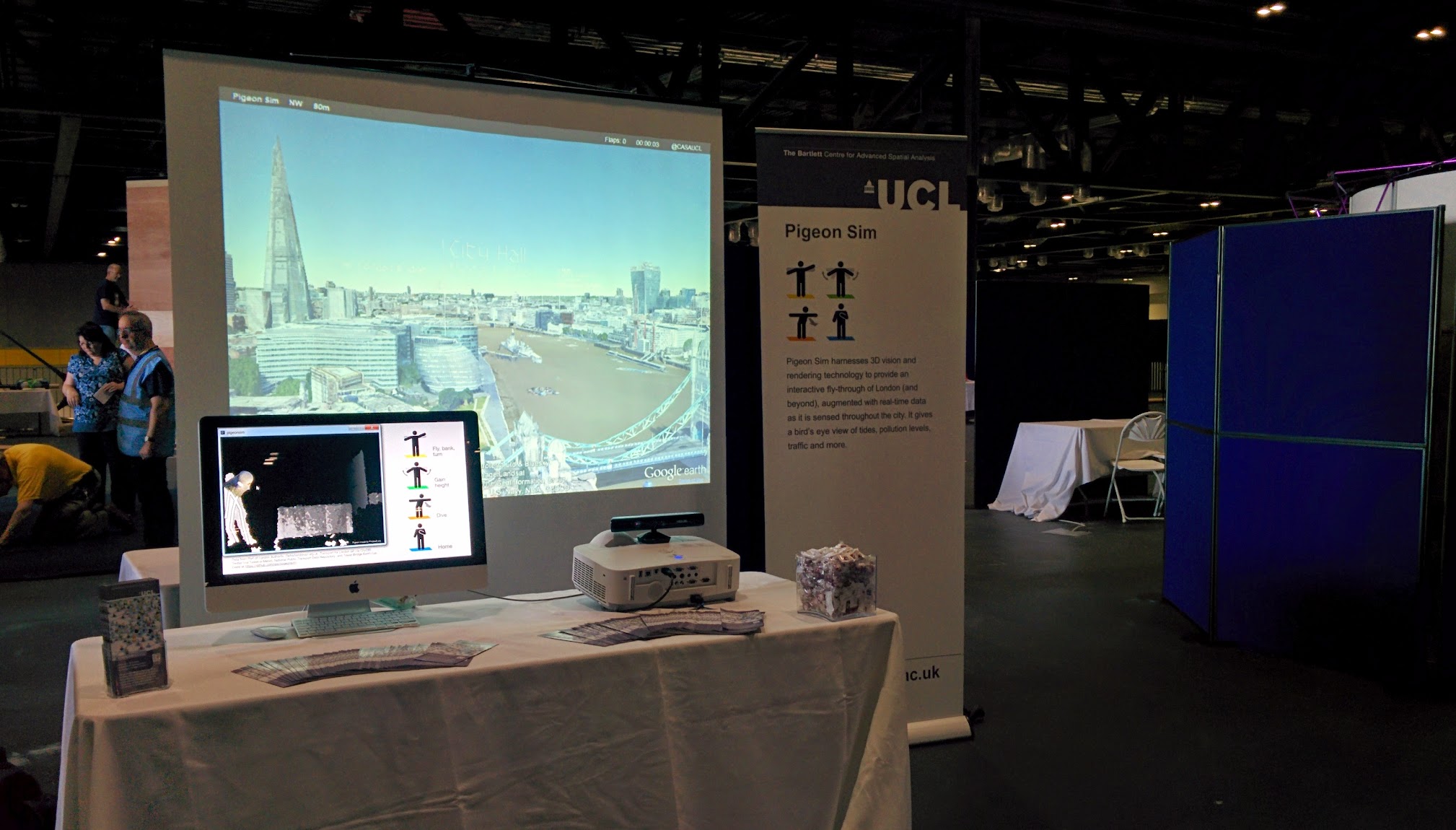
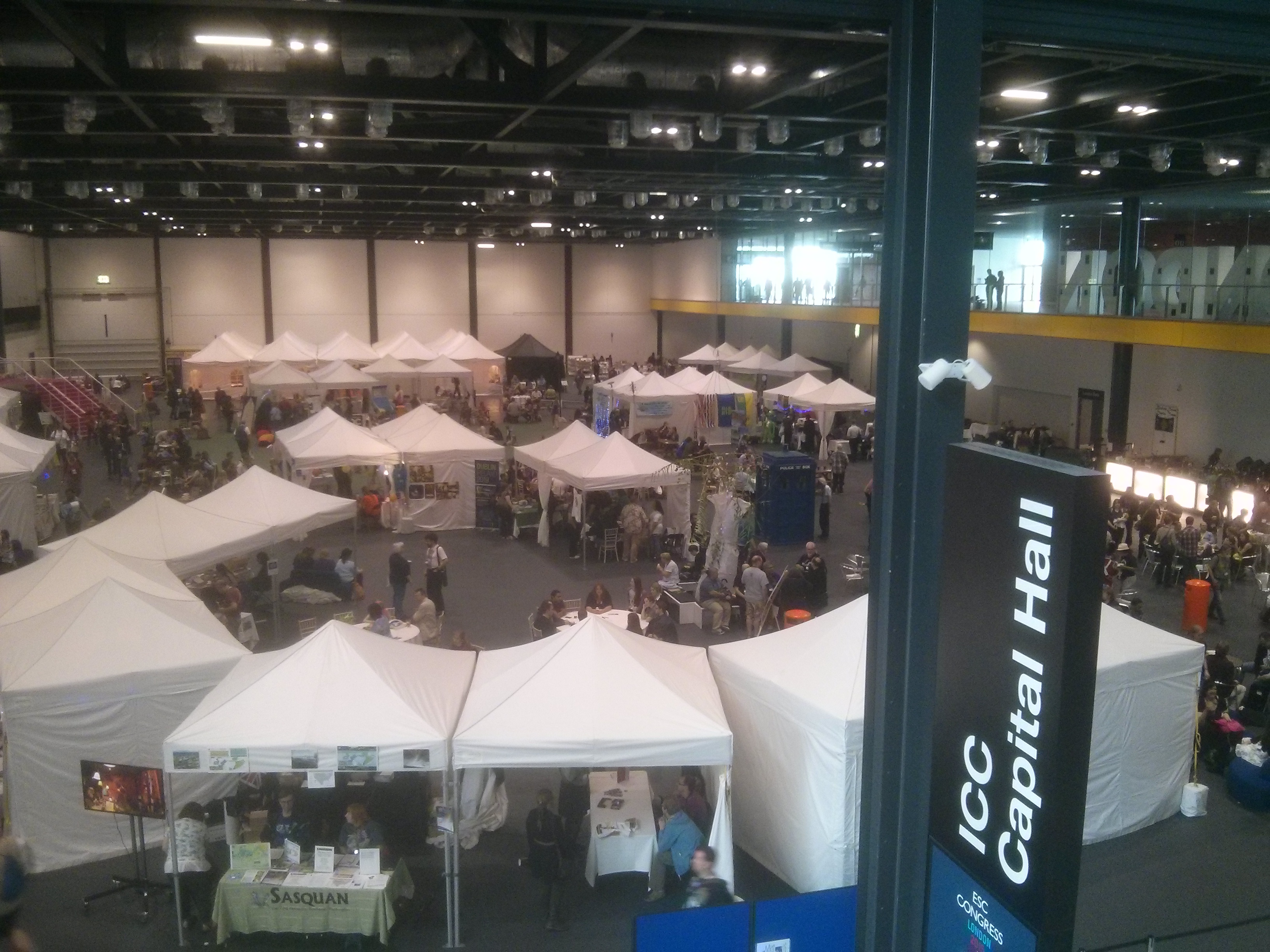
The pigeon sim visited the LonCon3 72nd World Science Fiction convention at the ExCeL centre last week. The event covered Thursday 14th to Monday 18th, with the weekend looking like the best part as lots of people were dressed up as science fiction characters. On the Friday shift we did get Thor on the pigeon sim, along with batman and spiderman though.
The picture above shows the build after Steve and Stephan had finished putting it all together on the Wednesday afternoon.
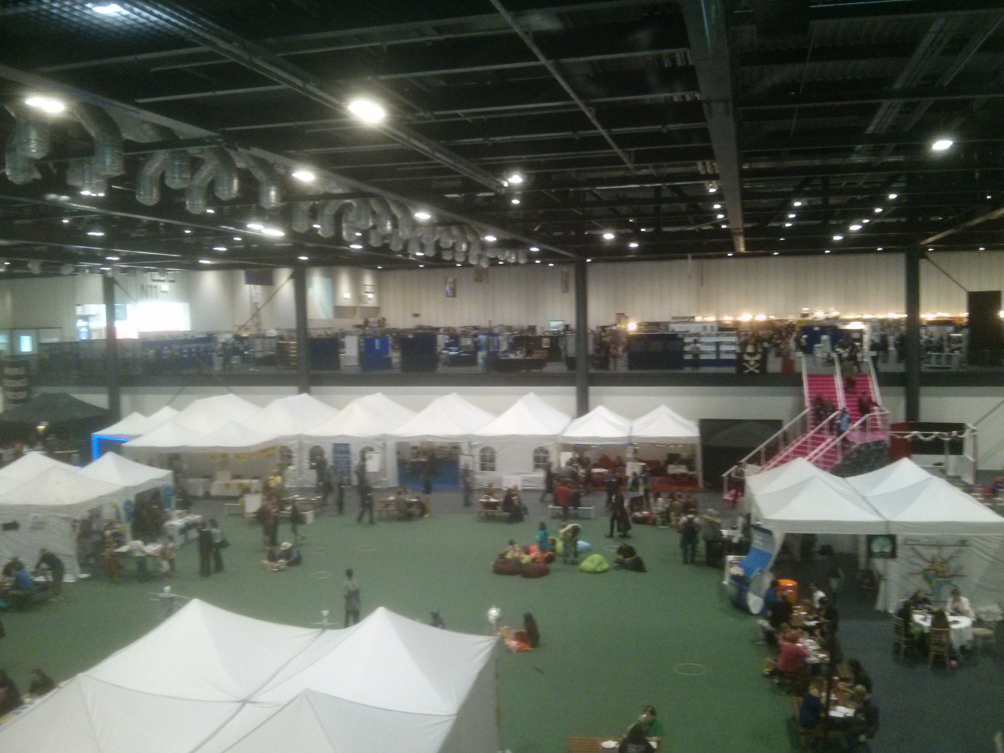
The white tents show the “village” area, while we were in the exhibitors’ area which is the elevated part at the top of the pink steps on the right. Our pigeon sim exhibit was about two rows behind the steps on the elevated level.
I’m slightly disappointed that Darwin’s pigeons (real live ones) weren’t arriving until Saturday, so I missed them, but the felt ones were very good:
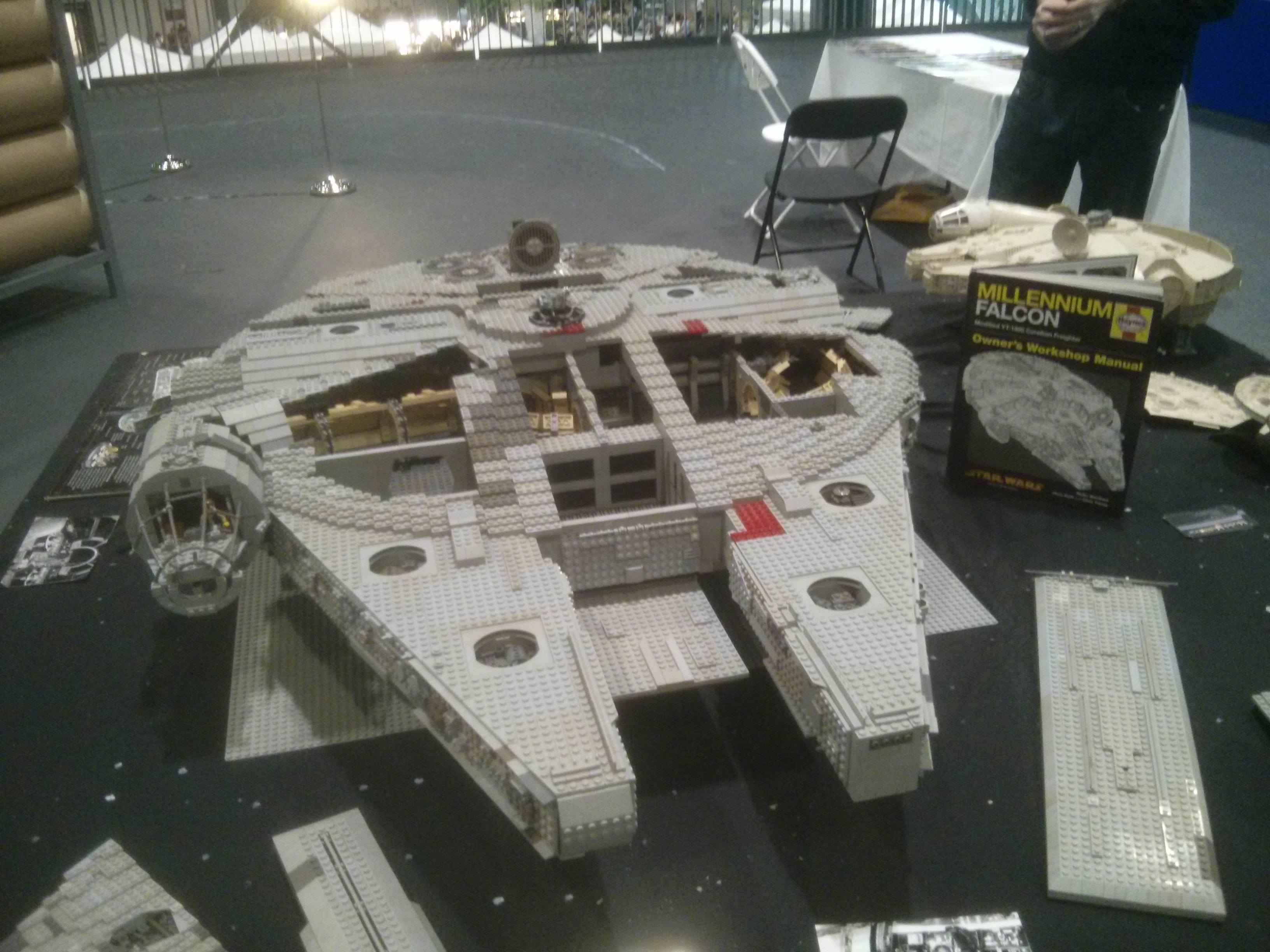
And finally, you can’t have a science fiction event without a Millennium Falcon made out of Lego:
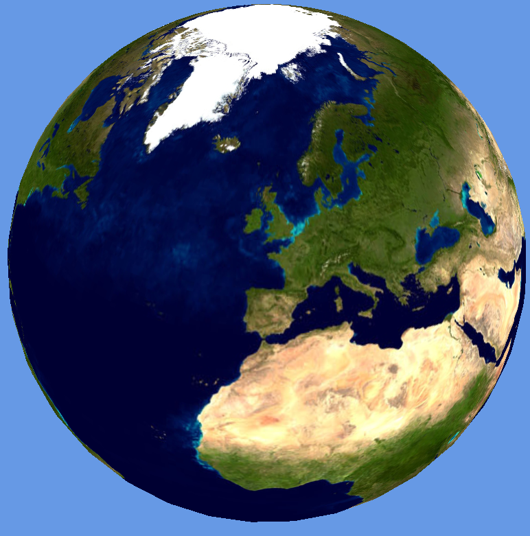
Following on from my last post about level of detail and Earth spheroids, here is the NASA Blue Marble texture applied to the Earth:
The top level texture is the older composite Blue Marble which shows blue oceans and a very well-defined North Pole ice sheet. Once the view zooms in, all subsequent levels of detail show the next generation Blue Marble from January 2004 with topography [link]. Incidentally, the numbers on the texture are the tile numbers in the format: Z_X_Y, where Z is the zoom level, so the higher the number, the more detailed the texture map. The green lines show the individual segments and textures used to make up the spheroid.
In order to create this, I’ve used the eight Blue Marble tiles which are each 21,600 pixels square, resulting in a full resolution texture which is 86,400 x 43,200 pixels. Rather than try and handle this all in one go, I’ve added the concept of “super-tiles” to my Java tiling program. The eight 21,600 pixel Blue Marble squares are the “super-tiles”, which themselves get tiled into a larger number of 1024 pixel quad tree squares which are used for the Earth textures. The Java class that I wrote to do this can be viewed here: ImageTiler.java. As you can probably see from the GitHub link, this is part of a bigger project which I was originally using to condition 3D building geometry for loading into the globe system. You can probably guess from this what the chunked LOD algorithms are going to be used for next?
Finally, one thing that has occurred to me is that tiling is a fundamental algorithm. Whether it’s cutting a huge texture into bits and wrapping it around a spheroid, or projecting 2D maps onto flat planes to make zoomable maps, the necessity to reduce detail to a manageable level is essential. Even the 3D content isn’t immune from tiling as we end up cutting geometry into chunks and using quad tree or oct tree algorithms. Part of the reason for this rests with the new graphics cards, which mean that progressive mesh algorithms like ROAM (Duchaineau et al) are no longer effective. Old progressive mesh algorithms would use CPU cycles to optimise a mesh before passing it on to the graphics card. The situation now with modern GPUs is that using a lot of CPU cycles to make a small improvement to a mesh before sending it to a powerful graphics card doesn’t result in a significant speed up. Chunked LOD works better, with blocks of geometry being loaded in and out of GPU memory as required. Add to this the fact that we’re working with geographic data and spatial indexing systems all the time and solutions to the level of detail problem start to present themselves.
The algorithms required to build virtual worlds like Google Earth and World Wind are really fascinating, but building a virtual world containing real-time city data is something that hasn’t yet been fully explored. Following on from the Smart Cities presentation in Oxford two weeks ago, I’ve taken the agent-based London Underground simulation and made some improvements to the graphics. While I’ve seen systems like Three.js, Unity and Ogre used for some very impressive 3D visualisations, what I wanted to do required a lower level API which allowed me to make some further optimisations.
Here is the London Underground simulation from the Oxford presentation:
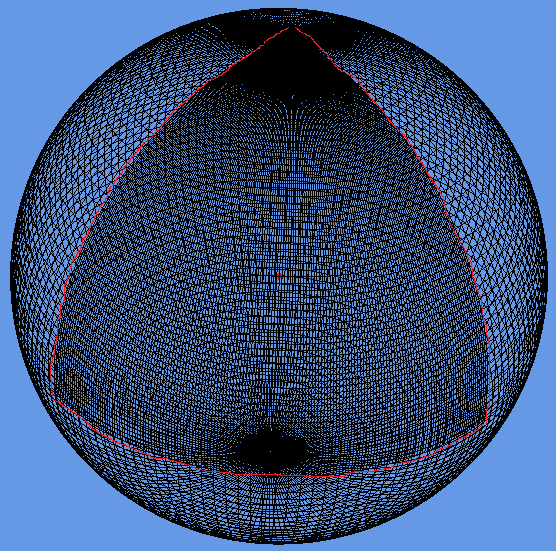
The Oxford NCRM presentation showed the Earth tiled with a single resolution NASA Blue Marble texture, which was apparent as the view zoomed in to London to show the tube network and the screen space resolution of the texture map decreased.
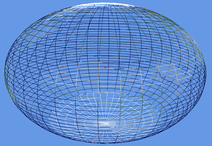
The Earth texture and shape needs some additional work, which is where “level of detail” (LOD) comes in. The key point here is that most of the work is done by the shader using chunked LOD. If the Earth is represented as a spheroid using, for example 40 width segments and 40 height slices, then recursively divided using either quadtree or octtree segmentation, we can draw a more detailed Earth model as the user zooms in. By using the same number of points for each sub-mesh, only a single index buffer is needed for all LODs and no texture coordinates or normals are used. The shader uses the geodetic latitude and longitude calculated from the Cartesian coordinates passed for rendering, along with the patch min and max coordinates, to get the texture coordinates for every texture tile.
The two images above show the Earth using the the NASA Blue Marble texture. The semi-major axis has been increased by 50%, which gives the “smartie” effect and serves to show the oblateness around the equator. The main reason for doing this was to get the coordinate systems and polygon winding around the poles correct.
In order for the level of detail to work, a screen space error tolerance constant (labelled Tau) is defined. The rendering of the tiled earth now works by starting at the top level and calculating a screen space error based on the space that the patch occupies on the screen. If this is greater than Tau, then the patch is split into its higher resolution children, which are then similarly tested for screen space error recursively. Once the screen space error is within the tolerance, Tau, then the patch is rendered.
The two images above show a correct rendering of the Earth, along with the underlying mesh. The wireframe shows a triangular patch on the Earth at the closest point to the viewer which is double the resolution (highlighted with red line). Octtree segmentation has been used for the LODs.
The code has been made as flexible as possible, allowing all the screen error tolerances, mesh slicing and quad/oct tree tiling to be configured to allow for as much experimentation as possible.
The interesting thing about writing a 3D system like this is that it shows that tiling is a fundamental operation in both 2D and 3D maps. In web-based mapping, 2D, maps are cut into tiles, which are usually 256 pixels square, to avoid having to load massive images onto the web browser. In 3D, the texture sizes might be bigger, but, bearing in mind that Google are reported to be storing around 70TB of texture data for the Earth, there is still the issue of out of core rendering. For the massive terrain rendering systems, management of data being moved between GPU buffers, main memory, local disk and the Internet is the key to performance. My feeling was that I would let Google do the massive terrain rendering and high resolution textures and just concentrate on building programmable worlds that allow exploration, simulation and experimentation with real data.
Finally, here’s a quick look at something new:
The tiled Earth mesh uses procedural generation to create the levels of detail, so, extending this idea to procedural cities, we can follow the “CGA Shape” methodology outlined in the “Procedural Modeling of Buildings” paper to create our own virtual cities.
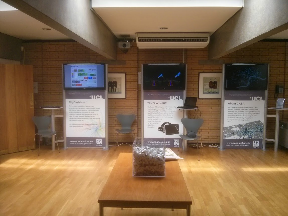
As you can see from the image below, we spent three days at the NCRM Research Methods Festival in Oxford (#RMF14) last week.
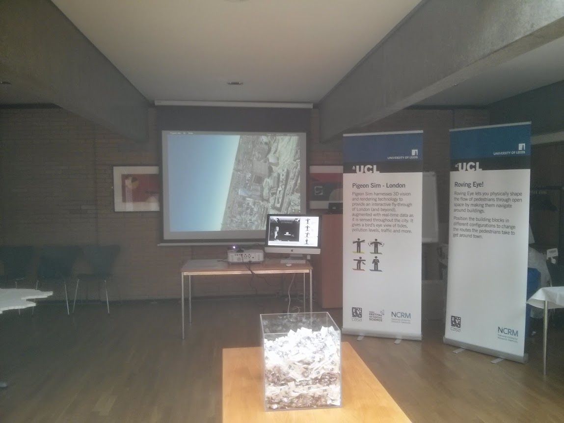
In addition to our presentations in the “Researching the City” session on the Wednesday morning, we were also running a Smart Cities exhibition throughout the festival showcasing how the research has been used to create live visualisations of a city. This included the now famous “Pigeon Simulator”, which allows people to fly around London and is always very popular. The “About CASA” screen on the right of the picture above showed a continuous movie loop of some of CASA’s work.
The exhibition was certainly very busy during the coffee breaks and, as always at these types of events, we had some very interesting conversations with people about the exhibits. One discussion with a lawyer about issues around anonymisation of Big Datasets and how you can’t do it in practice made me think about the huge amount of information that we have access to and what we can do with it. Also, the Oculus Rift 3D headset was very popular and over the three days we answered a lot of questions from psychology researchers about the kinds of experiments you could do with this type of device. The interesting thing is that people trying out the Oculus Rift for the first time tended to fall into one of three categories: can’t see the 3D at all, see 3D but with limited effect, or very vivid 3D experience with loss of balance. Personally, I think it’s part psychology and part eye-sight.
Next time I must remember to take pictures when there are people around, but the sweets box got down to 2 inches from the bottom, so it seems to have been quite popular.
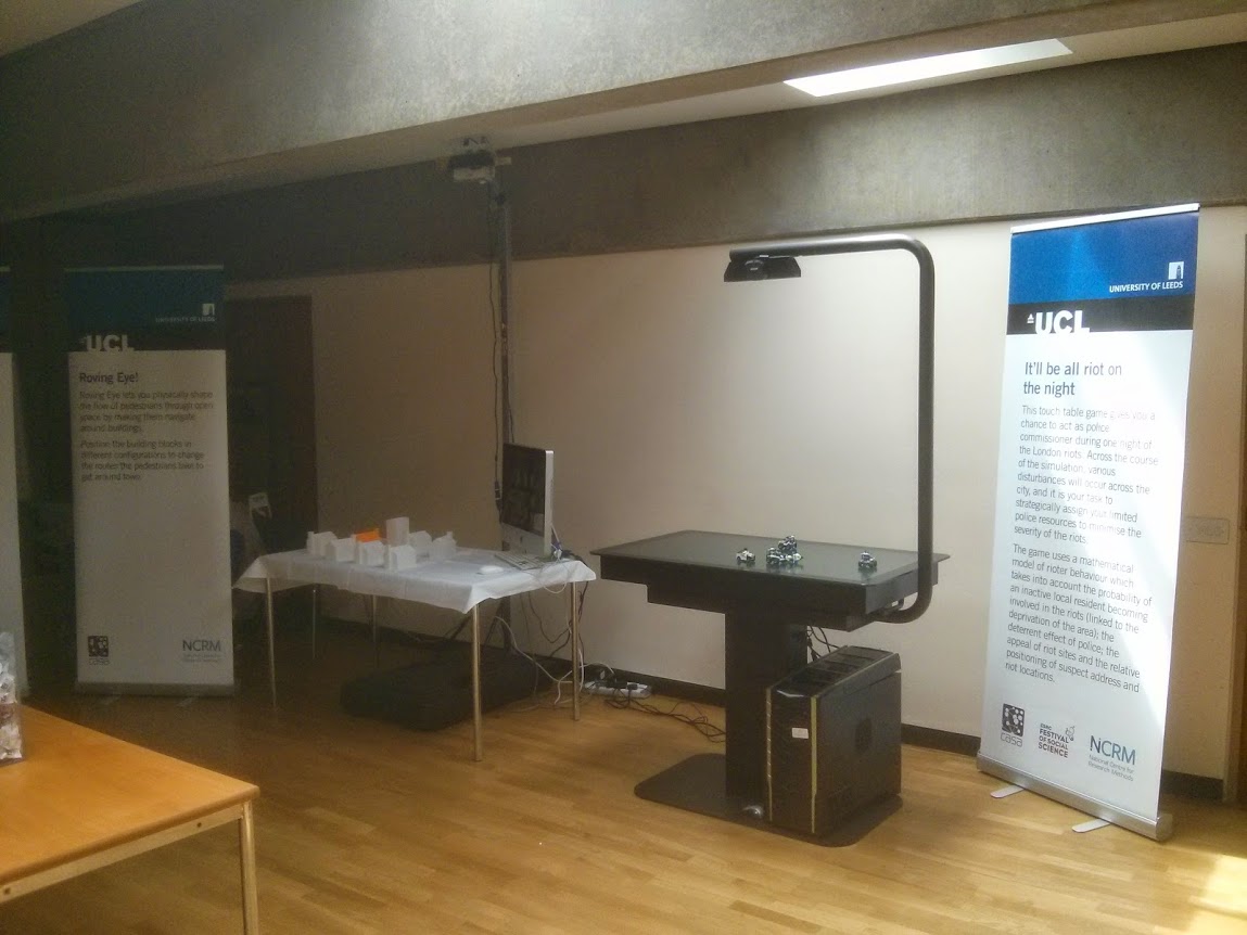
We had to get new Lego police cars for the London Riots Table (right), but the tactile nature of the Roving Eye exhibit (white table on the left) never fails to be popular. I’ve lost count of how many hours I’ve spent demonstrating this, but people always seem to go from “this is rubbish, pedestrians don’t behave like that”, through to “OK, now I get it, that’s really quite good”. The 3D printed houses also add an element of urban planning that wasn’t there when we used boxes wrapped in brown paper.
The iPad wall is shown on the left here with the London Data Table on the right. Both show a mix of real-time visualisation and archive animations. The “Bombs dropped during the Blitz” visualisation on the London Data Table which was created by Kate Jones (http://bombsight.org ) was very popular, as was the London Riots movie by Martin Austwick.
All in all, I think we had a fairly good footfall despite the sunshine, live Jazz band and wine reception.
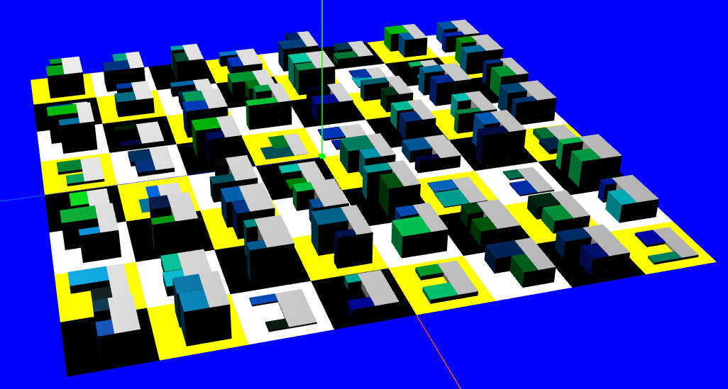
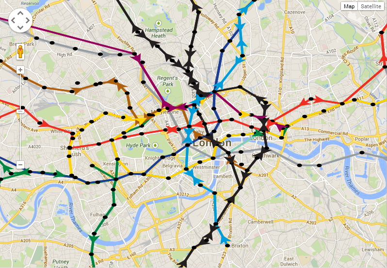
The image above is the position of all the tubes at 09:47 this morning, 29th April 2014.
As I was walking into work though, I was looking at the licence numbers of all the old Routemaster buses that TfL had put on as extra services. It’s a bus spotter’s paradise out there with all the old buses that are being driven around Central London. The problem, though, is that they don’t seem to have the same tracking devices on them as the regular buses, so they don’t appear on the Countdown API stream. This is potentially a big problem with collecting data on how the strike affects London, as we’re obviously missing some key information.
One good thing is that we now have access to road traffic data, so that might be worth analysing during tonight’s rush hour. Also, the people tracking project that I’ve been working on for a while is almost ready for testing.
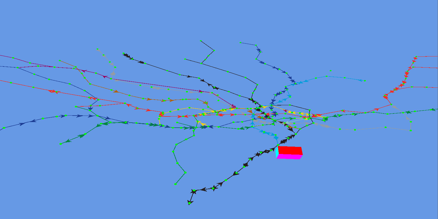
I’ve been getting increasingly frustrated with the tools available to visualise the tube, bus and train data I’ve been collecting, so I’ve ended up creating my own. If you’re wondering why some of the lines don’t have any tubes in the above diagram, it’s because I’ve got the speed set very high and I’m not picking the new route correctly when there is a choice.
The image above is an OpenGL visualisation in C++, but based on my experience with the AgentScript (2D) and Three.js (3D) browser based visualisations. Essentially, I wanted something that would allow me to create the animations that I’ve been using 3DS Max for, but in a much simpler way. The following is a bus animation that I built for a recent presentation:
This was created using 3DS Max, with some custom MaxScript code to load the bus positions and create the animation key frames. The main problem with this is the scale of the data, which is why I had to limit it to between 09:00 and 12:00. Art tools generally don’t like to handle this quantity of data and I’ve also had issues with packages like Unity and Lumion.
Increasingly, I’ve been moving towards the idea of “Programmable Maps” where the visualisation is built through a series of stages which load the data, apply behaviours to elements of the scene that move and produce an impressive 2D or 3D visualisation with advanced lighting or tilt shift in the same way as ViziCities. The use of APIs and 3rd party libraries to obtain the real-time data, along with the temporal aspect, makes it very difficult to fit this type of visualisation into a conventional GIS framework.
The example above is built around a C++ and OpenGL graphics engine, but one that is linked with geospatial libraries so it’s more than just a game engine rendering 3D assets as artwork. The experience with the XBox tubes demo (C#, XNA) and Chrome Three.js example showed that it’s a nightmare to get the geometry in the correct place and orientation unless it’s properly georeferenced. Working with the live tube data, where the API can only be queried every 3 minutes, leads to a real-time visualisation where positions are effectively being forecast between data updates. Putting all this together results in a requirement for a geospatially aware graphics engine linked with an agent based modelling package that allows us to code behaviours for the elements that are moving.
The programmable maps part doesn’t really come into play until you increase the level of sophistication and start to layer additional levels of processing. For example, bus positions are calculated based on arrival times at the next stop. This is a graph technique where you interpolate the time between nodes, but, in order to visualise the positions correctly, this position along the link needs to be applied to a road network to find the real position on the ground. Otherwise you get buses driving through the river and not using the bridges.
What I’m describing is a workflow for geospatial data to go from the raw data through to visualisation using library building blocks and web services where appropriate. There is one final trick to this approach though, as we could use it to make a visualisation directly from a NetLogo agent based model. A while ago I showed how to run the NetLogo program inside a Java program and capture the positions of the agents which can then be loaded into 3DS Max. Exactly the same thing could be applied here, with a NetLogo simulation driving the 3D engine.