Hex Bug Spiders with Computer Vision

Following on from my previous post about controlling the Hex Bug spiders from a computer, I’ve added a computer vision system using a cheap web cam to allow them to be tracked. The web cam that I’m using is a Logitech C270, but mainly because it was the cheapest one in the shop (£10).

I’ve added a red cardboard marker to the top of the spider and used the OpenCV library in Java through the JavaCV port. The reason for using Java was to allow for linking to agent based modelling software like NetLogo at a later date. You can’t see the web cam in the picture because it is suspended on the aluminium pole to the left, along with the projector and a Kinect. The picture shows the Hex Bug spider combined with Martin Austwick‘s Roving Eye exhibit from the CASA Smart Cities conference in April.

The Roving Eye exhibit is a Processing sketch running on the iMac which projects ‘eyeballs’ onto the table. It uses a Kinect camera so that the eyeballs avoid any physical objects placed on the table, for example a brown paper parcel or a Hex Bug spider.

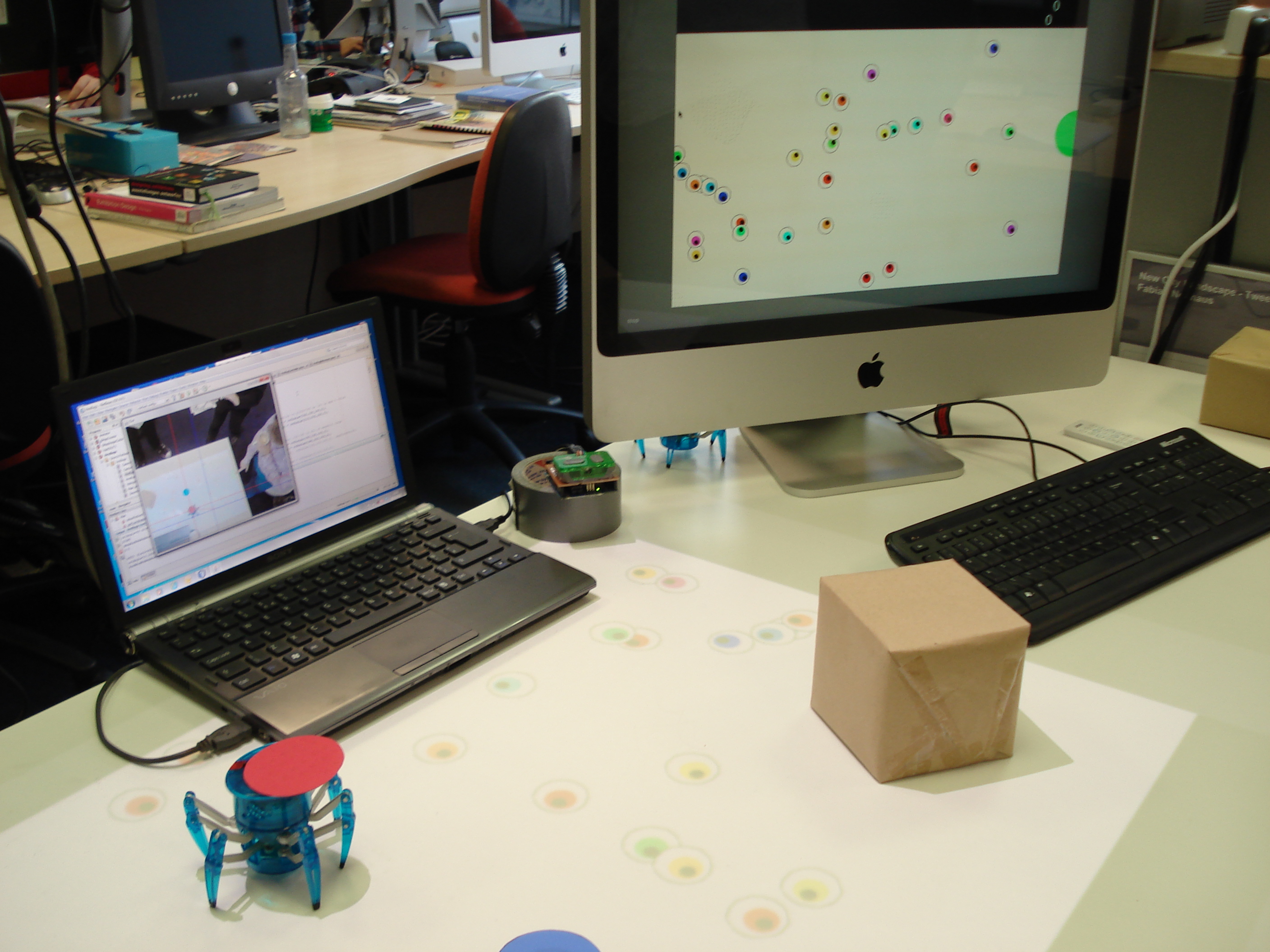
Because of time constraints I’ve used a very simple computer vision algorithm using moments to calculate the centre of red in the image (spider) and the centre of blue in the image (target). This is done by transforming the RGB image into HSV space and thresholding to get a red only image and a blue only image. Then the moments calculation is used to find the centres of the red and blue markers in camera space. In the image above you can see the laptop running the spider control software with the camera representation on the screen showing the spider and target locations.

Once the coordinates of the spider and target are known, a simple algorithm is used to make the spider home in on the blue marker. This is complicated by the fact that the orientation of the spider can’t be determined just from the image (as it’s a round dot), so I retain the track of the spider as it moves to determine its heading. The spider track and direction to target vectors are used to tell whether a left or right rotation command is required to head towards the target, but, as you can see from the following videos, the direction control is very crude.

The following videos show the system in action:


Links:

Martin Austwick’s Sociable Physics Blog: http://sociablephysics.wordpress.com/

Smart Cities Event at Leeds City Museum: http://www.geog.leeds.ac.uk/research/events/conferences/smart-cities-bridging-the-physical-digital/

Hacking Hex Bug Spiders

For the Smart Cities exhibition in Leeds in a couple of weeks, we’ve been building a physical representation of an agent based simulation. Hex Bug Spiders are relatively cheap hexapod robots that are controlled via an infra-red transmitter which has an A or B code so that you can control two simultaneously. The way it walks is referred to as the Jamius walking mechanism after its inventor (see: http://www.youtube.com/watch?v=is7x_atNl94 ).

After taking the Hex Bug apart the construction is actually really good for a cheap toy. Both the hand held transmitter and the receiver in the robot are based around the AT8EB one chip microcontroller  (Alpha Microelectronics Corp), with the robot itself also containing an ST1155A H Bridge driver. I’ve seen a lot of blog posts about hacking these spiders, but after trying to modify the robot’s control PCB to attach wires to the H Bridge driver directly (as in this blog post: http://www.instructables.com/id/Arduino-Controlled-Hexbug-Spider/), I’ve decided that it’s easier to replace all the electronics rather than hack the surface mount board. Out of the three spiders that I have, I’ve left two robots untouched while the third one has been disassembled. The logic behind this is to modify the IR transmitter and control two via an Arduino attached to a computer, while adding a ZigBee radio to the third for wireless control.

After examining the transmitter PCB, I noticed that there are exposed test points which can be used to attach wires for the forward, backward, left and right switches. I then discovered the following blog post doing almost exactly the same thing:

http://buildsmartrobots.ning.com/profiles/blogs/hack-a-hexbug-spider-for-serial-control-with-a-ti-launchpad

The following image shows the location of the test points on the front of the transmitter board:

The four test points for the forward, backward, left and right buttons are exposed, so it’s easy to solder on to them. I did have to very carefully remove some of the tape covering the button clickers first though. The A/B switch is very easy to solder to, but the + and – terminals from the battery are covered in hot melt glue which was very difficult to cut away. Then I had seven wires attached to the PCB which I routed through the A/B switch hole on the front case and re-assembled the transmitter. Reading from left to right, the white arrows identify the functions as follows: GND, Forward, +3.3V, Backward, (A/B code bottom with left above it), Right.

I have seen people connect Arduinos directly to the inputs of these transmitters, but, as I wasn’t happy connecting the 5v logic of the Arduino to the 3.3v logic of the AM8EB microprocessor, I used potential dividers on all the inputs. It’s never a good idea in microelectronics to have an input pin higher than Vss even if there are protection Zeners on the inputs.

The schematic of the final circuit is as follows:

(R1 to R5 are all 10K while R6 to R10 are all 15K. Apologies for the non-standard electronic symbols)

I have built this into an Arduino shield with the modified transmitter stuck onto the strip board using hot melt glue. This allows me to control two spiders via an Arduino connected via USB to a laptop. The laptop is running a Java program which uses the USB connection as a serial port to send single character commands to the Arduino which set the robot state as forward, backward, rotate left, rotate right or stop for two spiders (via the A/B code).

What I’ve found is that there needs to be about a 1 second delay after bringing up the serial port before you start sending commands to the robots, otherwise you lose the commands. While this does work to control two spiders from one transmitter using multiplexing on the Arduino to flip between the A and B codes, I think you really need two HexBug Arduino shields for it to work. By trial and error I found that holding the TX pins in spider A’s state for 80 ms, followed by the same for spider B, gave fairly reliable control of both simultaneously. Now that the project has progressed beyond the initial stages and we’re using a webcam to position the spider, this A/B code multiplexing is causing a lot of problems. The next phase involves getting the spider to follow a coloured marker and the only way I could get this to work reliably was to disable the A/B code multiplexing on the Arduino.

Transport Data During the Olympics

Having collected large amounts of data on tubes, trains and buses over the Olympics period using the ANTS library, the first thing I’ve looked at is to plot the total number of tubes running every day. The two graphs below show the number of tubes by line and the total number of tubes running for all lines.

Numbers of tubes running on each line from 25 July 2012 until 16 August 2012.


Total number of tubes running on all lines from 25 July 2012 to 16 August 2012. Weekend periods are highlighted with red bars.

Looking at this data it becomes apparent that the weekend has a very different characteristic compared to during the week. Also, there is a definite daily variation during the week with a distinct morning and evening rush hour. One interesting thing left to look at is whether the lines serving the Olympics venues show any variation before and during the Olympics period.

Smart Cities, Smart Transport?

I’ve described this as “radar for trains”, but it now also includes a real-time view of bus and tube delays. The idea is to produce a single visualisation highlighting where there are problems with the transport system:

Status of London’s transport system at 13:00 on 8 August 2012. The green squares are bus stops showing delays, while blue is for delays at tube stations.

The map above shows the fusion of all the sources of transport data gained from the ANTS project. Although we know the position of every tube, bus and train in London, simply plotting this information on a map tells you nothing about the current state of the city’s transport network. At any point in time there can be 450 tubes, 7,000 buses and 900 trains, so any real-time view needs to reduce the amount of information to only what is really significant.

London’s transport system at 13:00 on 8 August 2012 showing details about slow running buses on route 242 at the Museum Street stop

The data shown on the map is as follows:

1. National Rail trains more than 5 minutes late shown as red boxes, positioned at their last reported station.

2. Tube Stations where there is a wait of 20% more than normal, shown as blue boxes.

3. Bus Stops where there is a wait of 50% more than normal, shown as green boxes.

4. Segments of tube lines where the TfL status message indicates that there are problems, shown as red lines (there are none on this map).

The first problem with a system like this is that the data comes from three different sources, all of which are fundamentally different. Trains run to a very specific timetable, so you know it’s the 08:46 Waterloo train at Clapham Junction platform 10 and it’s running 6 minutes late. The map above does show the late trains as red boxes, but the Network Rail API is a stream, so it has to run for a period of time to pick up all the train movement messages. On the plus side though, we are getting information for every train in the country, but it quickly becomes apparent that there are a huge number of late trains, so we have to filter only those that are more than 5 minutes late.

When we get to the buses and tubes things get a bit more interesting as the information we get from the APIs isn’t linked to any timetable. In order to work out the delays, I’ve taken several months’ worth of archive data and computed an average wait time for every bus stop, tube station, platform and hour of day. Then what’s plotted on the map is any bus stop showing a wait more than 50% above average, or any tube station 20% above average for the current hour. In addition to this, if a section of tube line is flagged as having problems in the TfL status message, then this section will be highlighted on the map.

Mean wait time for every hour of the day (x-axis 0-23) computed for Oxford Circus, Northbound Platform, Victoria Line using archive data from November 2011 to July 2012

Looking at the mean wait time for Oxford Circus above, it’s possible to see the daily variation in tube frequency for the morning and evening rush hour (07:00-09:00 and 17:00-19:00), along with the overnight shutdown at 03:00 when the wait time is defaulted to zero.

Essentially, this is a data-mining and feature detection system, comparing what we normally expect to see with what’s happening now to highlight any differences. At the moment it’s using the mean wait time to detect problems, but it should probably use number of standard deviations from the mean. Now that we’ve got a working system we can start to look at the best methods for detecting problems and release this to the public once we’re happy with it.

Also see: the PLACR Transport API Website which does a similar thing for tube station wait times.

Tube Delays, Mean, Variance and Numerical Precision

This was something I came across while trying to calculate expected waiting times for tubes and buses. I’ve collected several months’ worth of transport data and wanted to calculate the mean and variance of waiting times at every station and platform. This can be achieved in a few hours for the tube, but there are over 600 bus routes in London and many more stops, so I needed something more computationally efficient than the naive algorithm that I was using.

After looking around, I found the following recurrance formulas for mean and variance:

[latex]M_k=M_{k-1}+(x_k-M_{k-1})/k[/latex]

[latex]S_k=S_{k-1}+(x_k-M_{k-1})*(x_k=M_k)[/latex]

See: http://www.jstor.org/stable/2286154 for a comparison of different methods, but the original method dates back to a paper from 1962 by B. P. Welford published in Technometrics: http://www.jstor.org/stable/1266577. It’s also in Donald Knuth’s book, “The Art of Computer Programming, Volume 2: Semi-Numerical Algorithms”, so I probably should have read my own copy a bit more carefully. The section on “Numerical Precision” in floating point maths is essential reading for any kind of data-mining or mathematical modelling. Not just because of the mantissa size and “Very big number minus very small number equals no change” problem, but also because I want to use running mean and variance to build an adaptive system that can detect problems in the transport network as they happen.

At the moment, the real-time problem detection system for the tube uses statistics that I have pre-computed, so when a waiting time at a station exceeds what is normal, then it gets flagged on the map as a potential problem. With the bus data calculations being so computationally intensive, it makes more sense to use the running mean and variance formulas in an online system so that it adapts over time to what is considered to be the normal operating point of the system.

The London Bus Strike: 22 June 2012

As part of the on-going ANTS project (Adaptive Networks for Complex Transport Systems) we’ve been tracking how many London buses are running during today’s bus strike. This is a very new development which we only just got working in time, so we don’t have any baseline data to compare against yet, but the two maps from this morning and lunchtime the day before show the geographical areas most affected by the strike.

Friday 22nd June 2012 09:00am showing the locations of buses as red markers with direction arrows

The above image shows all the buses running at 09:00am (BST) this morning when the strike was on. According to our data, there were 2,198 buses running in London at that time. We don’t yet have enough baseline data to compare this against, but by taking 13:21 (BST) on the previous day, we can say that there were 6,387 buses running then, giving 34% as a very rough guide.

Thursday 21 June 2012 13:18 (BST) showing the locations of buses as red markers with direction arrows

Comparing the two maps, it looks as though the worst affected area was the East of London. We can also show the density of buses using a heatmap:

Heatmap of bus locations for Friday 22nd June 2012 09:00 [Link to original map].

Following on from this, we also have data for the Underground, so this will enable us to analyse multi-modal flows and see how the bus strike has a knock-on effect on the tube.

Thanks to Steven Gray for drawing the bus icons as my original ones were useless.

ANTS: TfL Countdown API for Buses

The TfL Countdown API for buses was released a couple of weeks ago and I’ve been experimenting with it for the ANTS project so that we can add real-time bus tracking to the Tube, River Services and National Rail libraries. The ultimate aim of the ANTS project is to show how failures affect multi-modal flows, so integrating bus data into this system is the last major hurdle.

Buses on route 73, 17:22 on Monday 18th June 2012

The arrow icons need a bit of work as they are the ones I have been using to test the tube direction calculation code with, but they show which direction the bus is heading in quite effectively. In contrast to the tube data, the bus compass bearing is accessible from the API and seems to be taken directly from the GPS in the bus.

The position calculation is done by building up a passing points database of all the arrival times at bus stops as returned by the API. The aim was not to have to use any timetable data, or route data, so the locations can be calculated using only the data from the API. At the moment I’m only querying route 73 for debugging purposes, but the returned data contains the expected times of all buses for every stop along the route. This includes a unique trip code, a vehicle code and even the licence number of the actual bus. Unfortunately, the previous stop for a bus is missing, so we only know where the bus is heading, which makes interpolation along the route impossible. By building up the passing points database, we can query stopping points for the same bus route for a bus following behind the one we’re interested in and find out where it has come from. Then the position is a simple linear interpolation using the expected time, time now and run length for the link, also extracted from the passing points of a following service.

The London Transport Network in Realtime

Last Saturday, 5 May 2012, saw the FA Cup Final and various Olympics preparation events taking place in London, so I couldn’t help wondering was was going to happen to the transport system. The ANTS project (Adaptive Networks for complex Transport Systems) that I’ve been working on is designed as a toolkit for collecting transport data, so I used it to generate data for the Tube and National Rail networks. Now we have this data set, we can use it in other projects as an “FA Cup Final” scenario, allowing us to experiment on a real city.

The schedule of events for the day was as follows:

12:45 Arsenal played Norwich at the Emirates, attendance: 60,092

17:15 FA Cup Final between Liverpool and Chelsea at Wembley, attendance: 89,102

Evening, London Prepares Event at the Olympic Park, attendance: 40,000

5 May 2012 16:30 BST (45 mins before kickoff). Map shows tube locations taken from the TfL Trackernet API (link to raw data below)

The image above shows the positions of tube trains 45 minutes before the Cup Final kick off. Wembley stadium is located half way between the “y” of Wembley and the two tube lines above it, which is the location of the closest station to the ground, “Wembley Park” on the Metropolitan (purple) and Jubilee (grey) lines. It’s interesting to note the obvious gap in the service on the Bakerloo line (brown) which serves “North Wembley” and “Wembley Central” to the south (where the word “Wembley” cuts the brown line). We can look at the tube status messages from TfL for this time period and see that there are planned closures as follows:

District line (green): Turnham Green to Ealing Broadway

Northern Line (black): Camden Town to Mill Hill East and High Barnet

Piccadilly Line (dark blue): Acton Town to Uxbridge

These can be seen as sections on the map where there is an obvious lack of trains (open the KML links below for the original data containing station names). The significance of this is that any Chelsea supporters living around Turnham Green are going to get pushed towards Paddington to go North. Liverpool fans are likely to be coming from Euston.

If we move on to 20:30 after the Cup Final has finished and as the later events at the Olympic Park are starting, we can see the situation around Stratford (centre of map).

National Rail and Tube trains around Stratford for 20:30 (link to raw data below)

The National Rail trains show as blue, where the service is on time, red, where it is late, and white where the timetable shows there should be a service, but we can’t verify its location. Due to the differences in how National Rail services work, it is a completely different type of data to the Tube. For National Rail we can only look at the departure boards for stations and use the timetable to match up services. There is only one late train for this time period, coloured red and hiding in the top left corner. This highlights the differences in the type of data as it takes several minutes to query enough data from National Rail to make the map, during which time the trains move around, causing the uncertainty in the data.

This is still a work in progress and requires a much more rigorous analysis, but you can see delays occurring around Wembley just before and after the match, plus some services heading for Stratford running a couple of minutes late in the evening. I’ve not got any information on the National Rail closure affecting services back to Liverpool in the evening, but it doesn’t look as if they were any really major problems.

As this was the first attempt at collecting a comprehensive set of data for a single day, it didn’t go completely to plan. There are questions about how you cope with the uncertainties in the National Rail data and how you compare it with the Trackernet information. The DLR and Overground are missing, as are the buses and it’s not clear how to use the TfL tube status information. We also don’t know anything about the commuters on the network, so can only guess at where all their journeys begin and what route they take. What is also needed is baseline data on what a normal Saturday should look like, which will give us the ability to pull anything abnormal out of the data.

Ultimately, the reason behind doing this is to provide a real-time snapshot of London’s transport network and how it behaves over the course of a day. For this we need to establish an automatic method of detecting and highlighting problems which is proving difficult at the moment. Then we can look at how a problem on one line has a knock-on effect on another.

The image below shows an animation of all tube trains for the 16 April 2012 from 8am to 8pm [link to movie]:

Links to data used in this post:

Tube Network KML

Trackernet 16:30 KML

National Rail 20:24 KML

Trackernet 20:30 KML

MapTube Map of Realtime Tube Locations

MapTube Topical Maps

It is four years today since MapTube was launched at the Barbican and to mark this event, I’ve made some changes to how the home page displays. This is a bit of an experiment, but I’ve tried to make the home page display topical data by using RSS feeds from the BBC News page, the Guardian and our own CASA blog aggregator. The basic method is to construct a list of keywords and frequencies from the RSS feeds, removing any words on a “stop words” list like “a”, “and”, “or” etc. Then a network graph of MapTube’s maps is constructed where each vertex is a map which is linked by edges made from where maps share keywords. So, for example, all the “London” maps form a fully connected group. This is similar to my previous post on using “Force Directed Graphs for Visualisation of Search Results”: http://talisman.blogweb.casa.ucl.ac.uk/2012/01/23/force-directed-graphs-for-visualisation-of-search-results/

Network Graph of MapTube London Maps

Once the connections between the maps has been calculated, each vertex is visited in turn and assigned a topicality value based on the RSS word frequency of all the map’s matching keywords. This weight is then propagated through the network via any connected edges up to a distance of 2 links from the parent vertex, with the weight reduced by a factor of 1/(r^2), where “r” is the number of vertices traversed. I did experiment with how many links from the parent vertex to travel, but found that 1 or 2 links from the parent gave the best results. Any further than this and it just ends up giving weight to the maps with the highest number of connections.

As I stated at the beginning, this is still very much an experiment and I’ve deliberately built the system with enough degrees of freedom to allow for some tinkering with the algorithm. I can control which feeds we mine for the topical keywords, the stop words list can be edited (I had to put “us” back in as we have a lot of United States maps) and I also have the ability to add my own keyword weights. At the moment I’ve artificially inflated the real-time tube locations map to get it onto the front page along with our most popular map of the London Underground tube station locations, which is now three years old. The first run of the system on the live server produced high values for a lot of the air quality maps, which was an interesting result.

The biggest criticism I had of MapTube was that the home page always displayed the most popular maps, sorted by the number of hits. This meant that the most popular maps stayed on the front page by virtue of people always clicking on the top ones. We did try showing the most recently added maps for a while, but that didn’t work as lots of test maps get uploaded with no data on them. Hopefully, as this new topical maps system evolves, we should see MapTube as a much more dynamic source of geographical information.

One final point, but by knowing what data we have on MapTube that’s topical, we also know what’s topical that we don’t have and should perhaps try to track down and upload. This approach would form a closed loop geographic information system.

National Rail Train Locations

The purpose of my previous post on the TransXChange timetable data was to make it possible to track National Rail trains in real time. Due to the large number of stations making up the network and the fact that you can’t obtain information for a whole line in one go, the only viable option is to use timetable data. The other limiting factor is the lack of any kind of unique train identifier on the National Rail website (see: http://ojp.nationalrail.co.uk/service/ldbboard/dep/EUS ).

The preliminary results are shown below:

Trains going into or out of Waterloo for 16:42 on a weekday

The technique is quite simple and involves making requests to the National Rail website to probe the current positions of trains. We first ask where the trains should be at the current point in time based on the timetable. Then, we probe the running information for the stations just ahead of where the trains should be. Tested using the whole of the Greater London network, only 319 unique station requests were required to determine train positions out of a total of 2,575 stations. This number can be reduced even further as we only need to hit on a single station ahead of the train in order to find out whether it’s on time. The position can always be worked out from the timetable by asking where it should be on its route at the time now minus the late minutes.

Once all the data for the departure boards has been collected, the next stage is to match up trains to departure details for stations based on the passing points extracted from the TransXChange timetable. This links a train to the running service which tells us all the stopping points and times on its route, along with a unique route code. This unique route code is used to identify the same train on different departure boards so we can use the best position information available, in other words, the departure board that it is approaching next.

An interesting question is what happens if there is enough of a disruption to the services to make the timetable useless? In this situation, the concept of whether a train is late is meaningless, but we still have a system which can probe the departure boards and match trains using the runtimes between stations. Certain network geometries make it impossible to match trains accurately without timetable data if the destination is shared between two routes. For example, a “Y” section where two trains with the same destination code merge onto one line. Another complicating factor is the circular route, where trains all start at Waterloo and end up at Waterloo again.